Check in igraph how to identify particular routes in a network

Analyzing the graph using igraph

library(igraph)
library(tidyverse)

igraph is versatile to analyze network properties. The first step is to create an igraph object from the edge list and node list tha comes out of Mark´s app

Mucor_edge<-read.csv("processedData\\DF56(6)_t09-Edge.csv",header = T, stringsAsFactors = F)#Node_Traits[which(Node_Traits$name=="DF56(6)_t09"),]
Mucor_node<-read.csv("processedData\\DF56(6)_t09-Node.csv",header = T, stringsAsFactors = F,sep = ";",dec = ",")#Node_Traits[which(Node_Traits$name=="DF56(6)_t09"),]

edges_1<-Mucor_edge[,c("EndNodes_1","EndNodes_2")]#Edge_Traits[which(Edge_Traits$name=="DF56(6)_t09"),c("EndNodes_1","EndNodes_2")]
edges_1<-graph_from_edgelist(as.matrix(edges_1),directed = F)

spatial.data<-Mucor_node[,#Node_Traits[which(Node_Traits$name=="DF56(6)_t09"),
                          c("node_ID","node_X_pix","node_Y_pix")]

l <- as.matrix(spatial.data[,c(2,3)])
l <- norm_coords(l, ymin=-1, ymax=1, xmin=-1, xmax=1)

Visualizing the network via the igraph object

plot(edges_1,
     edge.arrow.size=1,edge.curved=0,edge.width=2,
     edge.color="black", vertex.label=NA,vertex.shape="none",
     edge.size=150,vertex.size=0,layout=l*1,main="Real Network")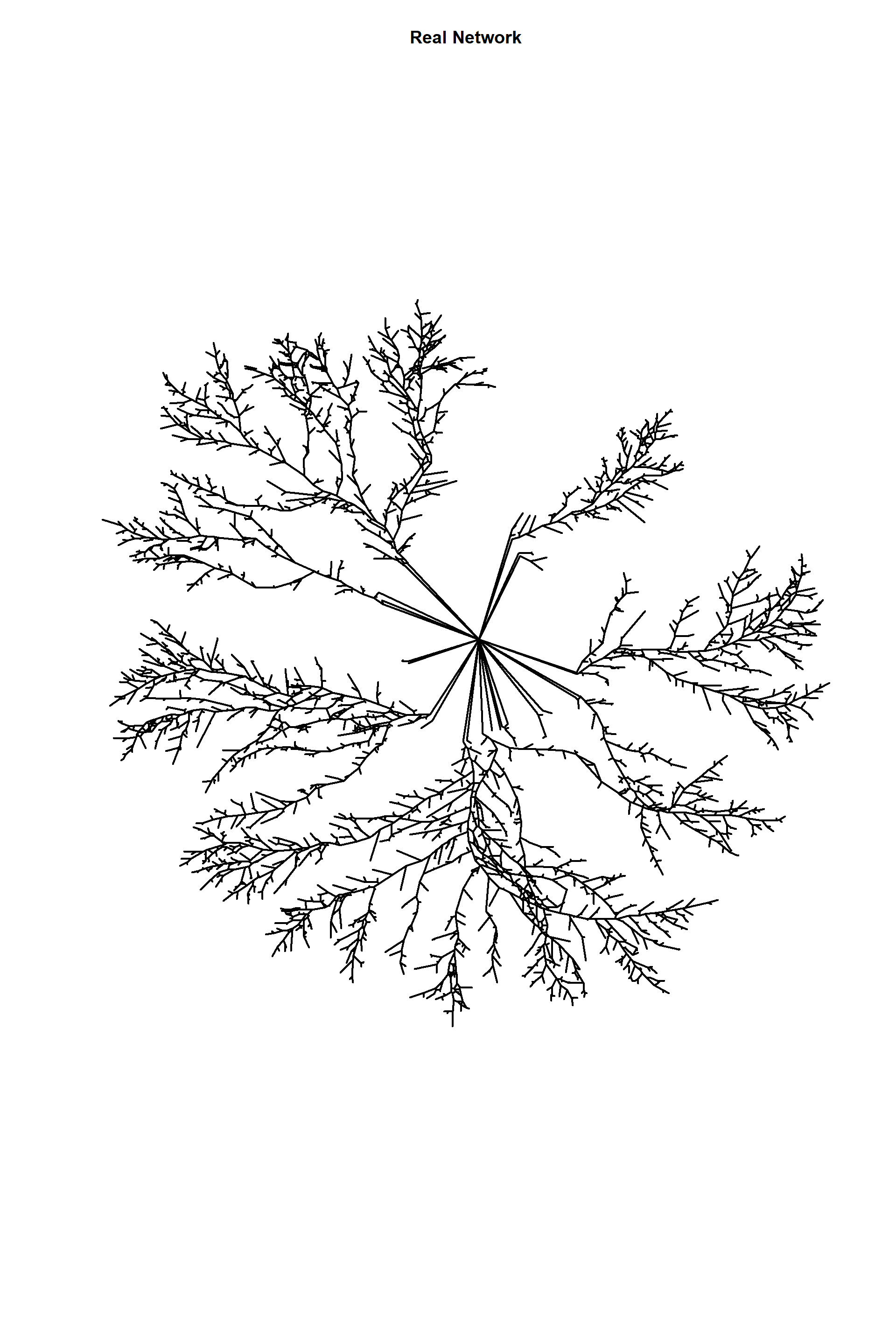

Assigning attributes to the igraph object

Attributes can be anything and can be name however I want to. Except for “weight” which will be used as the link weight

According to Mark´s manual these weights for hypha should be resistance. Other than those I will assign other attributes: length, width, distance for hyphae; same thing can be done to nodes

#E(edges_1)$weight<-Mucor_edge$Resistance_2ave
E(edges_1)$weight<-Mucor_edge$Resistance_2
E(edges_1)$lenght<-Mucor_edge$Length
E(edges_1)$width<-Mucor_edge$Width
V(edges_1)$degree<-degree(edges_1)
V(edges_1)$distance<-Mucor_node$node_Distance
E(edges_1)$distance<-Mucor_edge$Distance


#NOTE!!!!!
#tapply(Edge_Traits$Width,Edge_Traits$name,max)#This is weird the maximum is fixed at 5.6 regardless of the colony, and when I also analyze my close up, I also get 5.6 as max value (which particularly makes no sense)
#tapply(Edge_Traits$Width,Edge_Traits$name,min)

Calculating the shortests paths

Now I calculate the shortests paths from the inoculum and to every other vertex. As specifed in Mark´s manual, the shortest path is the one that sums the lowest resistance (using Resistance_2). To do this, igrap has the function get.shortest.paths, which according to its documentation uses the same algorithm as reported in Mark´s manual, quoting: “By default igraph tries to select the fastest suitable algorithm. If there are no weights, then an unweighted breadth-first search is used, otherwise if all weights are positive, then Dijkstra’s algorithm is used.”

#With this line one can check which number corresponds to the inoculum
Mucor_edge[which(Mucor_edge$Type=="F"),c("EndNodes_1","EndNodes_2")]

##      EndNodes_1 EndNodes_2
## 2761       2390       5279
## 2777       2405       5279
## 2796       2419       5279
## 3013       2601       5279
## 3048       2629       5279
## 3054       2635       5279
## 3062       2640       5279
## 3354       2875       5279
## 3392       2906       5279
## 3678       3155       5279
## 3692       3171       5279
## 3823       3272       5279
## 3900       3338       5279
## 3950       3382       5279
## 3967       3397       5279
## 4004       3430       5279
## 4015       3437       5279
## 4018       3439       5279
## 4030       3451       5279
## 4067       3485       5279
## 4083       3496       5279
## 4249       3626       5279
## 4300       3668       5279
## 4470       3822       5279
## 4472       3823       5279
## 4476       3826       5279
## 4489       3840       5279

trial<-get.shortest.paths(edges_1,from = 5279)

I can now get node accessibility using igraph. For that I use the function distances and it does give me exactly the same values as in node_accessiblity coming from Mark´s app

plot(
distances(edges_1,v=5279),#here each distance is the lowest summation of edge resistances from node 5279 to each other node
Mucor_node$node_Accessibility
)

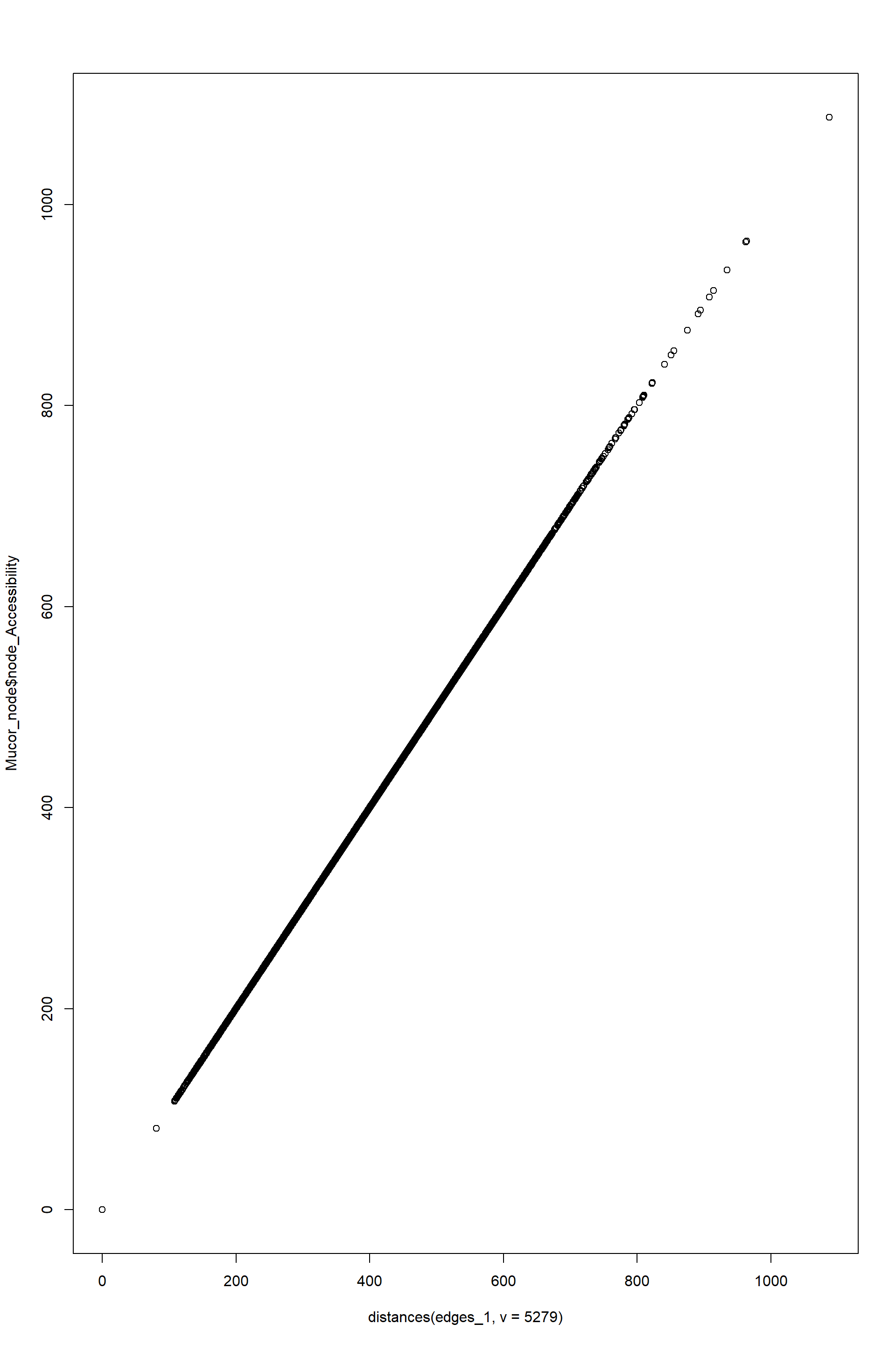
temporal<-distances(edges_1,v=5279)
summary(as.vector(temporal)/
as.vector(Mucor_node$node_Accessibility))

##    Min. 1st Qu.  Median    Mean 3rd Qu.    Max.    NA's 
##       1       1       1       1       1       1       1

Now I am trying to get the total length of those shortests paths. In principle these lenghts should be identical to the ones obtained by multiplying the node route factor with the node distance

(Mucor_node$node_RF*Mucor_node$node_Distance)[1]

## [1] 5358.125

I found two methods to do this:

#Method 1
sum(E(edges_1,path = trial$vpath[[1]])$lenght
    )

## [1] 5427.525

#Method 2
sum(
E(induced.subgraph(edges_1,as_ids(trial$vpath[[1]])))$lenght
)

## [1] 5427.525

Now calculating these lengths for all the network using method 1 and comparing with node_rf * node_distance

route_lengths<-rep(0,length(Mucor_node$node_RF))
for (i in 1:length(trial$vpath)) {
  route_lengths[i]<-sum(E(edges_1,path = trial$vpath[[i]])$lenght
    
  )
}

plot(
  (Mucor_node$node_RF*Mucor_node$node_Distance),
  route_lengths
)

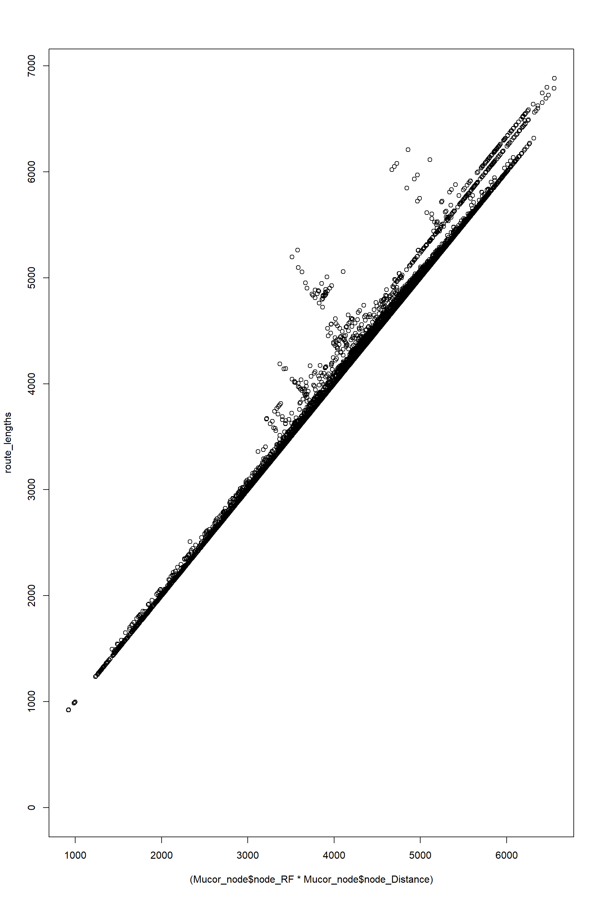
A smilar result is obtanied by using method 2 and comparing with node_rf * node_distance

These results confirm the following:

igraph calculate distances based on hyphal resistance using the Dijkestra algorithm exactly in the same way as in Mark´s app. This means that accessibility to a node is simply the lowest summation of resistances of edges (a path) from the inoculum to that node.
Also that the accessibility produced by the app is based on resitance_2 (I tried with resistance_2ave and the match is good but not exact)
But for some reason there is small discrepancy between the lengths calulation. I think that the culprit might be in the values of length themselves, but his would need to be checked.

Now trying to calculate new stuff

Here, what I am doing is selecting a particular “shortest” path based on their width. This means that one can select distincts parts of the mycelia for analysis.

ecol<-rep("black",ecount(edges_1))
ecol[
   E(edges_1,path = trial$vpath[[1]])[
      E(edges_1,path = trial$vpath[[1]])>=0.7*
         E(edges_1,path = trial$vpath[[1]])$width]
   ]<-"orange"

plot(edges_1,
     edge.arrow.size=1,edge.curved=0,edge.width=2,
     vertex.label=NA,vertex.shape="none",
     edge.color=ecol,
     edge.size=150,vertex.size=0,layout=l*1,main="Real Network")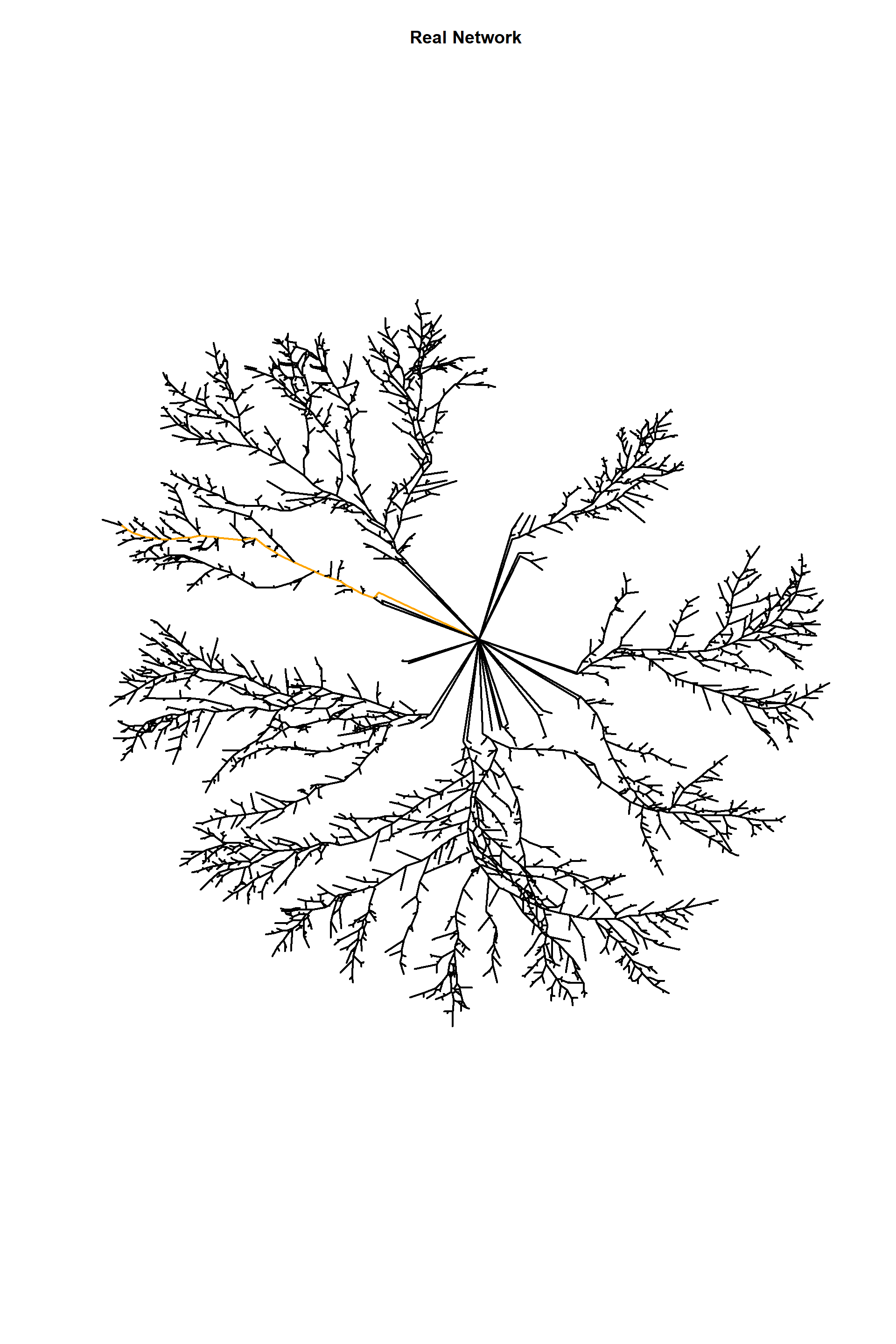

#neighbors(edges_1,5279)
#incident(edges_1,5279)

E(edges_1)$type<-"E"
E(edges_1)[incident(edges_1,5279)]$type<-"F"

ecol<-rep("black",ecount(edges_1))
ecol[
  E(edges_1)$lenght==max(
E(edges_1)[
E(edges_1)$type=="E"]$lenght)
   ]<-"orange"

plot(edges_1,
     edge.arrow.size=1,edge.curved=0,edge.width=2,
     vertex.label=NA,vertex.shape="none",
     edge.color=ecol,
     edge.size=150,vertex.size=0,layout=l*1,main="Real Network")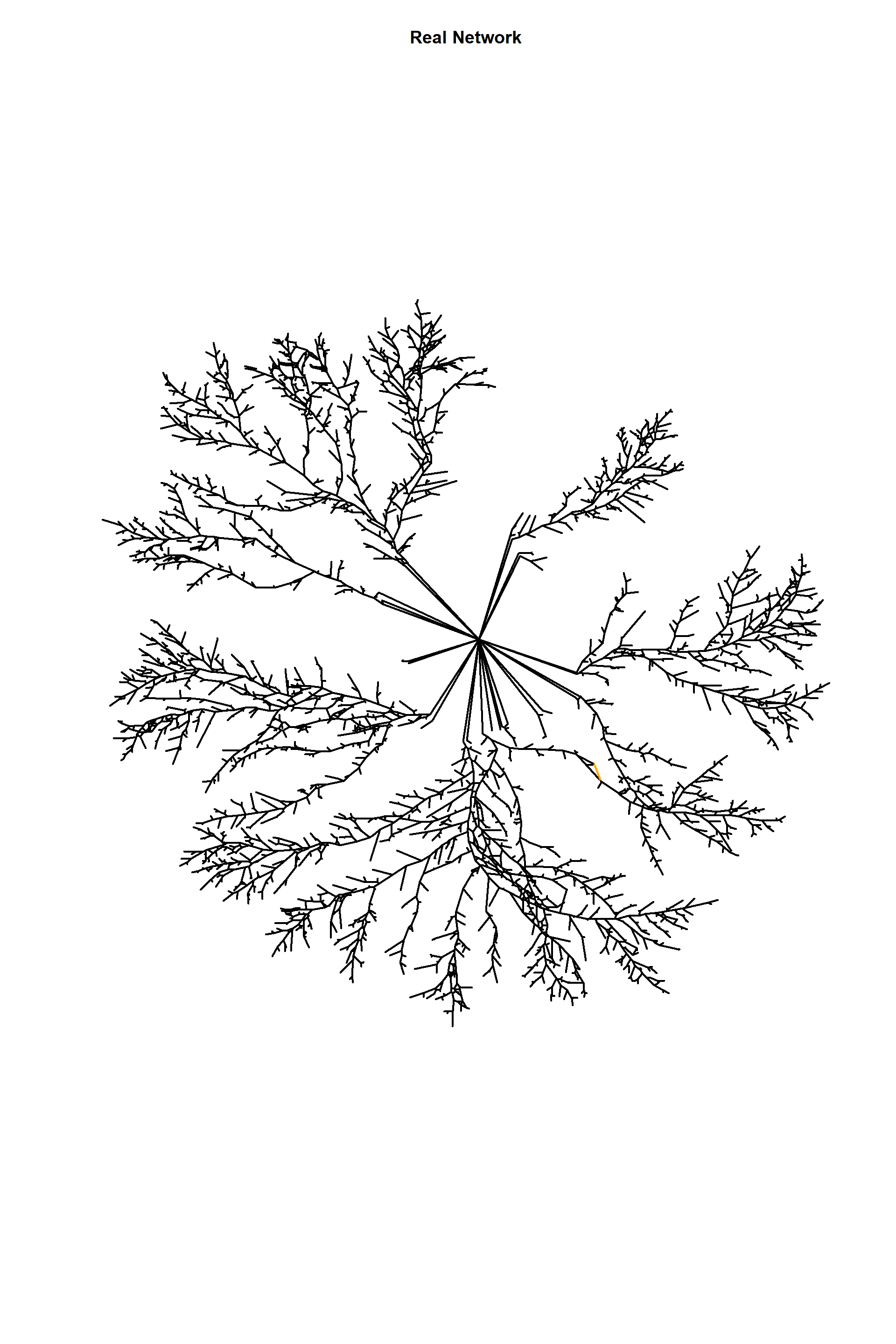

ecol<-rep("black",ecount(edges_1))

ecol[E(edges_1)[inc(V(edges_1)[degree==1])&lenght>200]#Selecting very long hyphal tips
  ]<-"green"

ecol[E(edges_1)$type=="F"]<-"gray80"

# ecol[E(edges_1)[inc(V(edges_1)[degree==2])]
#   ]<-"blue"
# ecol[E(edges_1)[inc(V(edges_1)[degree==3])]
#   ]<-"red"

plot(edges_1,
     edge.arrow.size=1,edge.curved=0,edge.width=2,
     vertex.label.cex=0.2,
     #vertex.shape="none",
     edge.color=ecol,
     edge.size=150,vertex.size=0,layout=l*1,main="Real Network")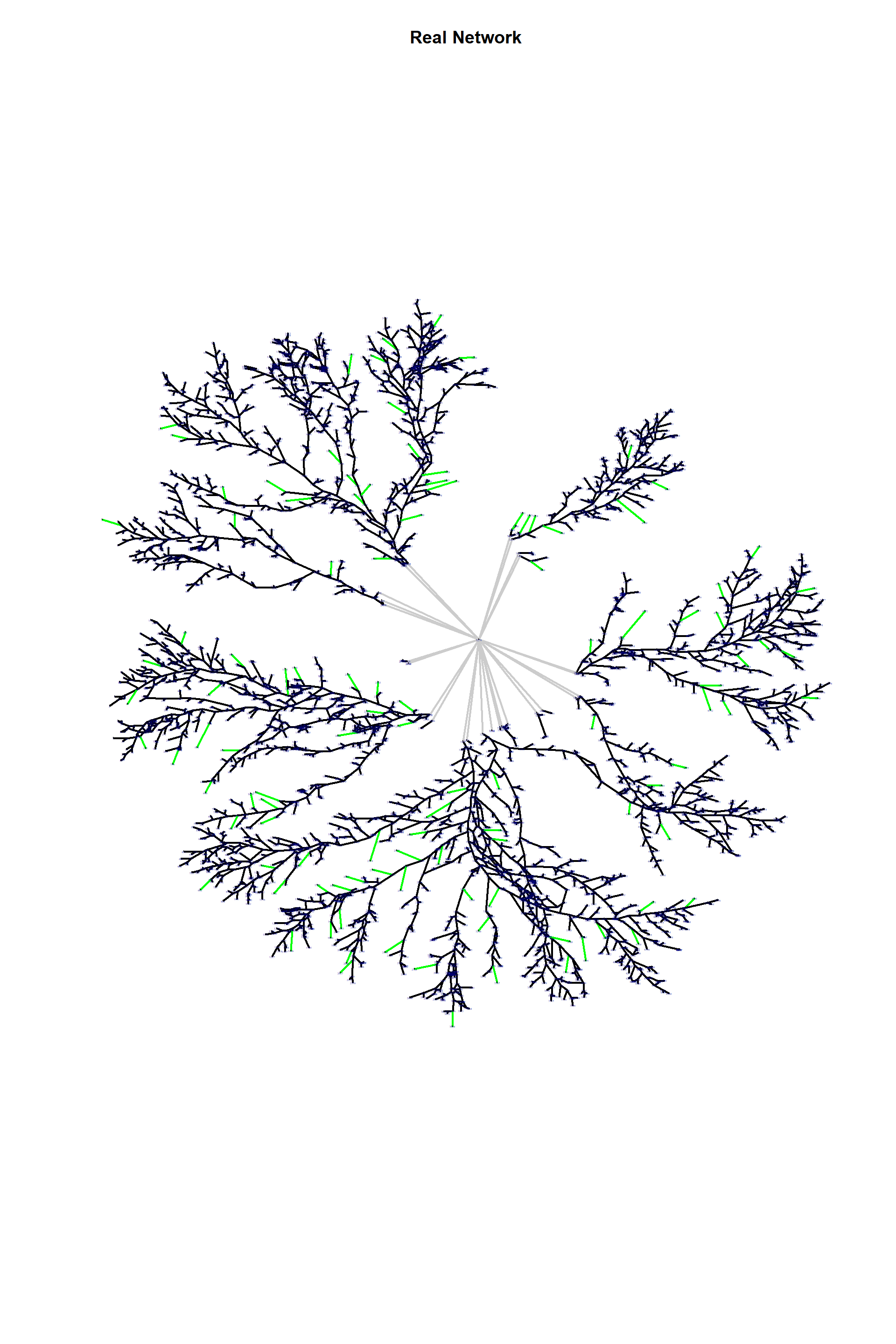

# plot(edges_1,
#      vertex.label.color="black", vertex.label.cex=1,vertex.size=1,
#      edge.color=ecol,layout=l)
#

Obtaining toy networks and calculating similar variables as in the the real networks

Minimum weighted spanning trees

edges_1mst<-mst(edges_1)

head(E(edges_1mst)$weight)

## [1] 166.918838  12.880956  14.951232   9.968187  11.853373  29.209799

length(E(edges_1))

## [1] 6090

length(E(edges_1mst))

## [1] 5278

plot(edges_1mst,
     edge.arrow.size=1,edge.curved=0,edge.width=2,
     edge.color="black", vertex.label=NA,vertex.shape="none",
     edge.size=150,vertex.size=0,layout=l*1,main="Minimum Spanning Tree")

Minimum euclidean spanning trees

edges_1_no_weights<-edges_1

edges_1_no_weights<-
delete_edge_attr(edges_1_no_weights,"weight")

edges_1_no_weights_mst<-mst(edges_1_no_weights)

length(E(edges_1_no_weights_mst))

## [1] 5278

E(edges_1_no_weights_mst)$weight

## NULL

plot(edges_1_no_weights_mst,
     edge.arrow.size=1,edge.curved=0,edge.width=2,
     edge.color="black", vertex.label=NA,vertex.shape="none",
     edge.size=150,vertex.size=0,layout=l*1,main="Minimum Spanning Tree no weights")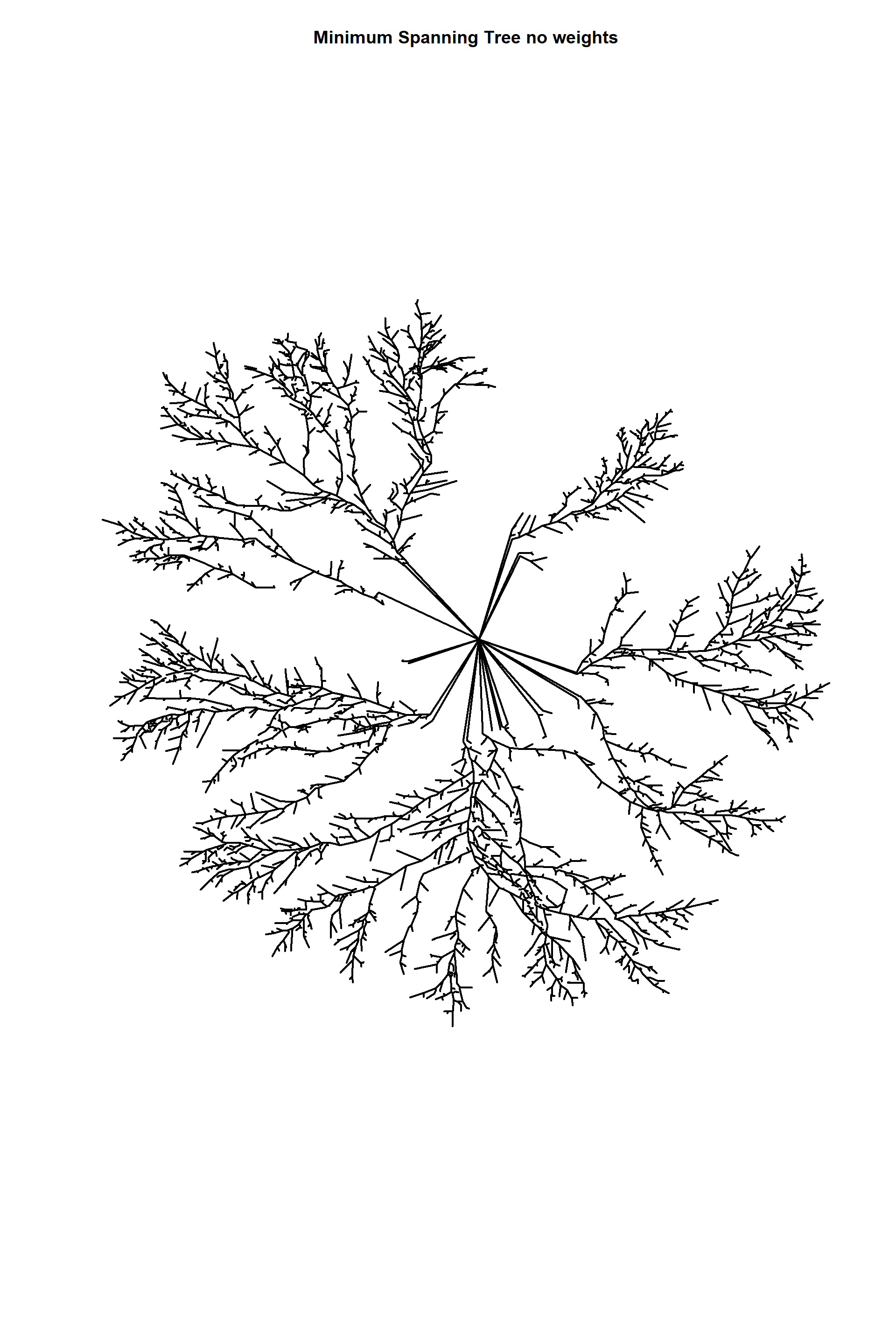

For the other toy models (like the relative neighborhood graphs, gabriel graph and delauney triangulation) it seems it is more complicated because they are based on vertex positions not based on network attributes. One possiblity would be to add weights to the toy models based on mean attribute values from the real models and then calculate resistance and accessibility

Comparing widths of tips and “main” hyphae based on node degree

no_feature<-
subgraph.edges(edges_1,E(edges_1)[type=="E"])

E(no_feature)$hyphae<-"main"
E(no_feature)[inc(V(no_feature)[degree==1])]$hyphae<-"tip"
#E(no_feature)[inc(V(no_feature)[degree==1])]$hyphae<-"tip"

probando<-rbind(
  
data.frame(degree="tip",Lengths=
E(no_feature)[hyphae=="tip"]$lenght,
Widths=E(no_feature)[hyphae=="tip"]$width,
Distance=E(no_feature)[hyphae=="tip"]$distance),

data.frame(degree="main",Lengths=
E(no_feature)[hyphae=="main"]$lenght,
Widths=E(no_feature)[hyphae=="main"]$width,
Distance=E(no_feature)[hyphae=="main"]$distance)#,

)

#table(probando$degree)

probando %>% 
  #filter(degree=="main") %>% 
  ggplot()+
  aes(degree,Widths)+
  geom_boxplot()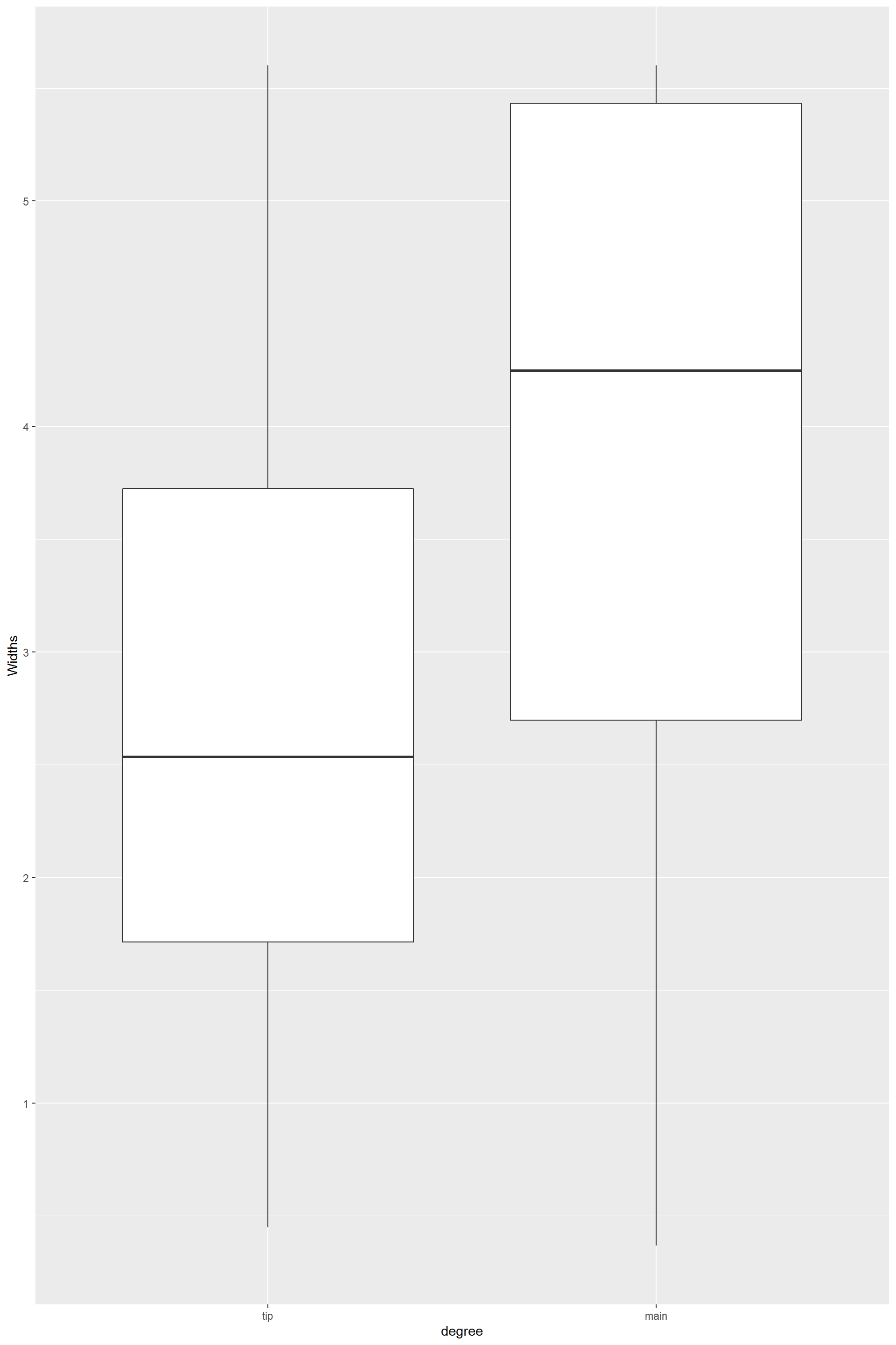

  #aes(Distance,Widths)+#It does not seem to be a relationship between widht and distances, meaning that certain hyphae remian thick all the way from the inoculum to the the tip
  #geom_point()

hist(probando$Widths[probando$degree=="main"])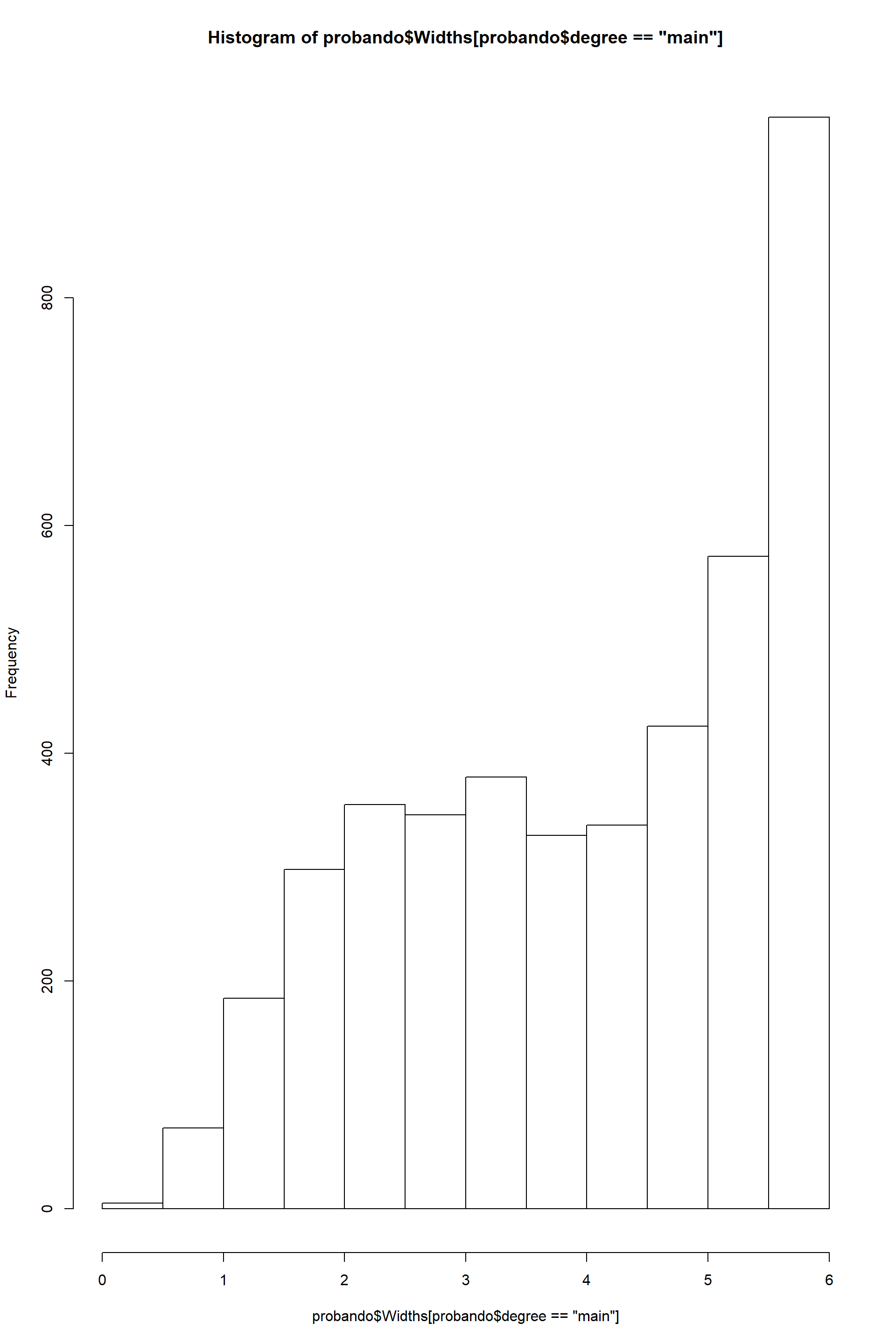

hist(probando$Widths[probando$degree=="tip"])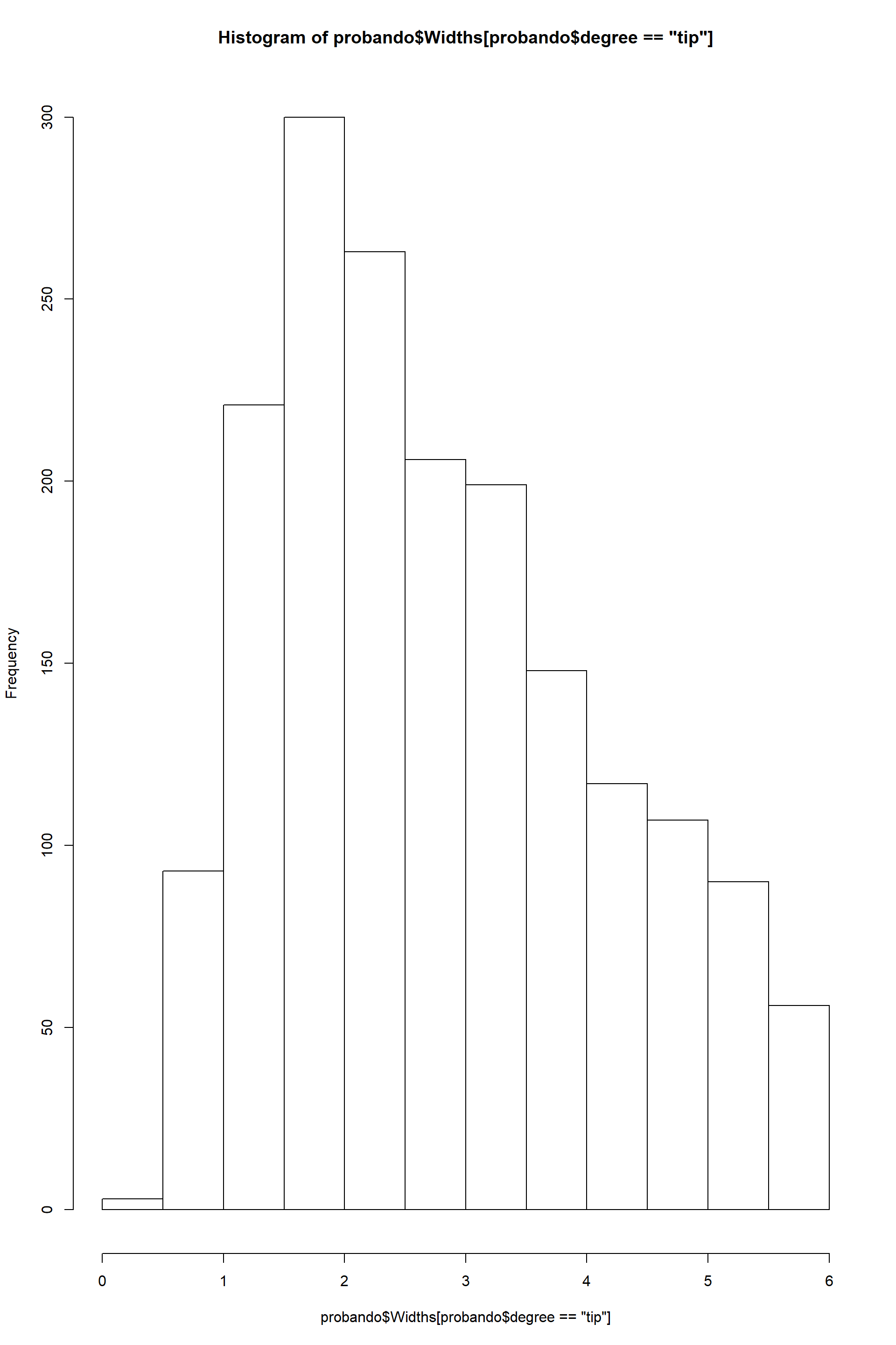

From these plots it is clear that there is a difference in width between hyphae a the tips and main hyphae. But that is not the case for length, which keeps constant along the mycelium. So as descriptive trait I will use each mean for width and a single mean for length

Left overs

Analyzing hyphal width as a bimodal distribution. This was deprepecated in favour of separate analysis of hyphal tip widths and main hyphae widths distinguishing them by degree
Understanding betweeness. This analysis was deprecated. Instead I move all analysis of network traits using igraph. But some patterns are interesting:
The betwenness of edges k=1 is not the same as the total number of edges
But these two values are proportional to each other
The edges of maximum betweenness for each colony are located always close to the center of the colony
But they are not at the minimal distance, they lay though within 2 times the minimum distance
It makes sense for the maximum betweenness to lay close to the center of the colony as it is where most of the “root” edges are
The minimum betweenness value is 0 and it occurs in all colonies. Thus the question is, what do edges with betwenness 0 have in common?

+ a) They are not tips. All of them have a degree larger or equal to two

1. They represent between the 6% to 14% of all edges

analysis with igraph